Columbia University Irving Medical Center
Transforming human health by driving discovery, advancing care and educating leaders

Our Schools
Advancing Care
News
- April 19, 2024
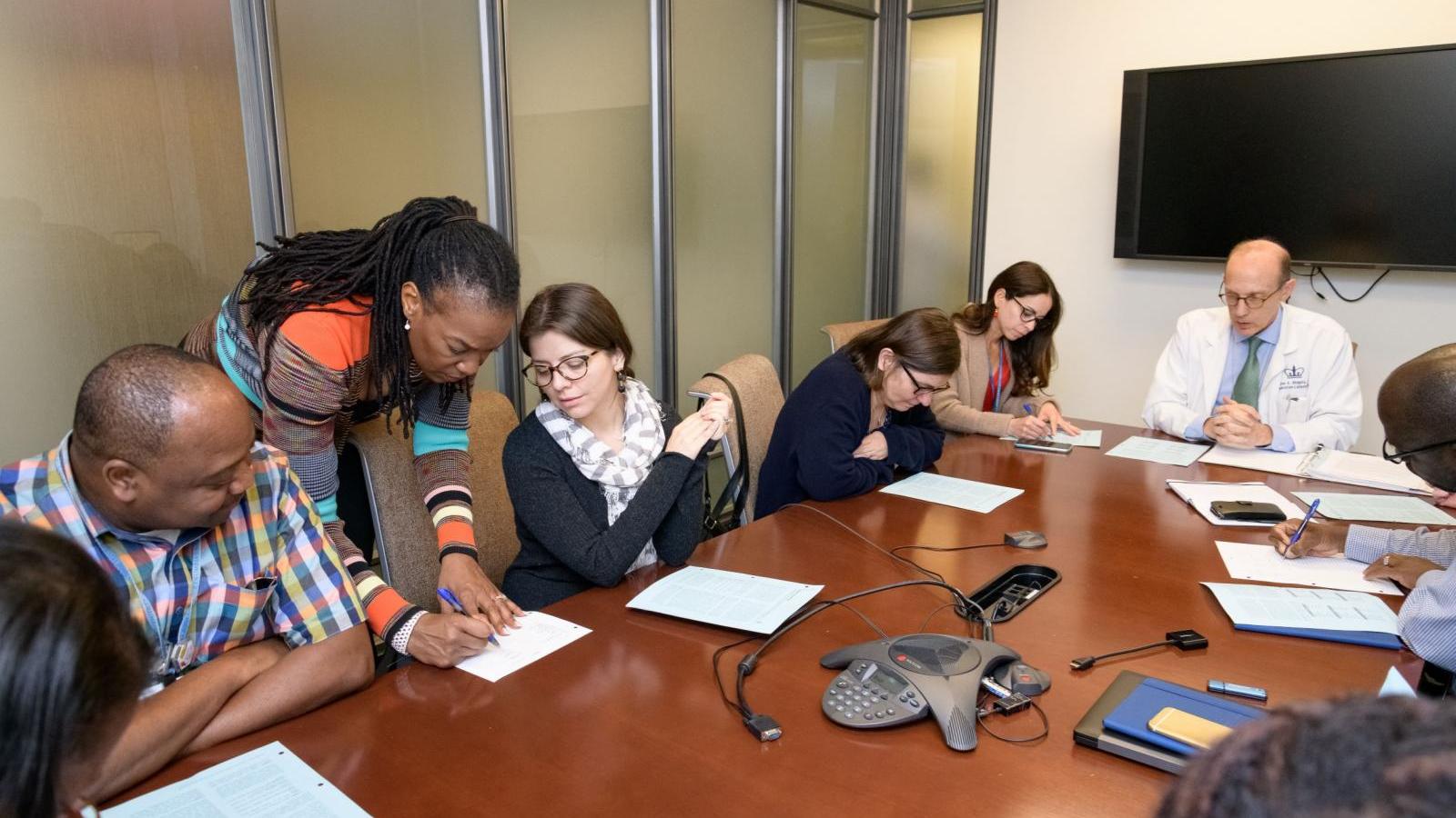
The new Center for Innovative Exposomics in the Mailman School of Public Health s positioned to be a major player in this rapidly emerging field.
Topic
- April 4, 2024
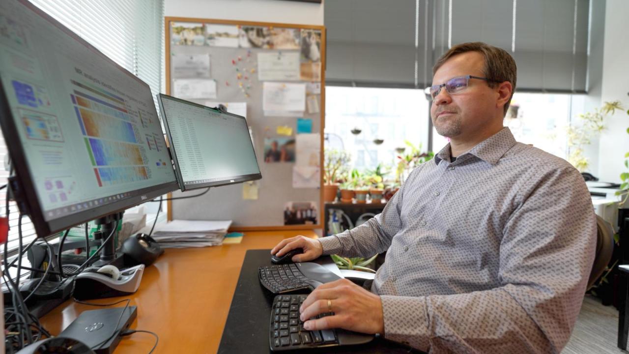
Radiology is leading the way on the translation of AI tools into the clinic and cancer screening may be the first area to benefit.
Topic
- April 3, 2024
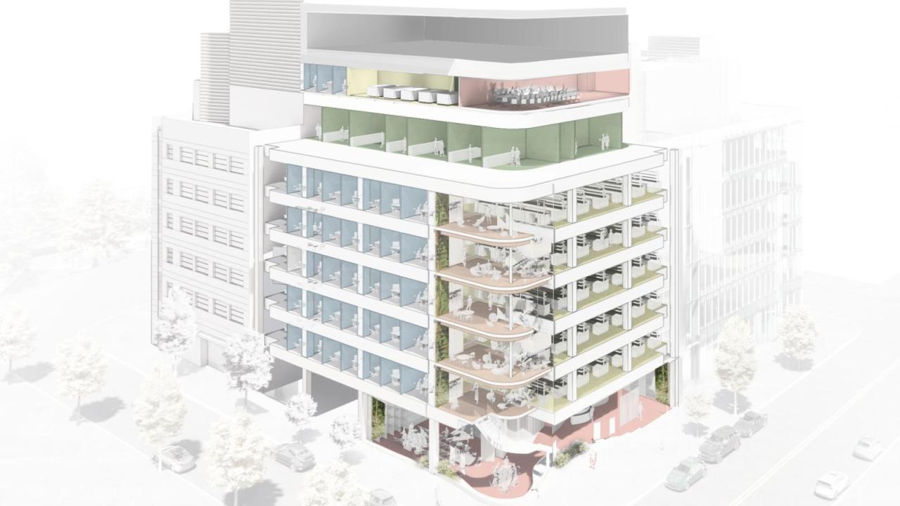
Columbia will begin construction in May on New York City’s first all-electric university research building.
Topic
- April 9, 2024
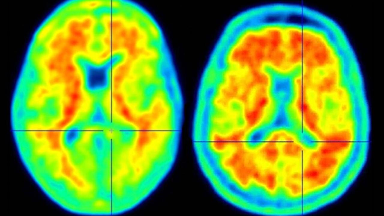
Columbia neuroscientists have identified a genetic mutation that fends off Alzheimer's in people at high risk and could lead to a new way to protect people from the disease.
Topic
- April 8, 2024
A new type of investigational therapeutic for pancreatic cancer has shown unprecedented tumor-fighting abilities in preclinical models of the disease.
Topic


Our Community

Learn more about our role in serving the Northern Manhattan community of Washington Heights, Inwood, and Harlem.
Diversity, Equity, and Inclusion
At CUIMC, we are committed to providing culturally inclusive medical education, research, and clinical care.
Events
- Friday, April 19, 20241:00 PM to 6:00 PM
- Saturday, April 20, 202410:00 AM to 5:00 PM
- Monday, April 22, 202411:45 AM to 12:45 PM
- Monday, April 22, 20243:00 PM to 4:00 PM
Venue
Online